Iceberg Classification Challenge
This notebook is my baseline entry into the ongoing kaggle iceberg data contest.

Introduction
Is it a ship or is it an iceberg? This project processes synthetic-aperture radar images and uses machine learning to identify whether each image contains a ship or an iceberg. Sounds easy enough, right? Well, the images are not normal images:
Synthetic aperture radar (SAR) images are captured from a moving antenna emitting successive pulses of radio waves. Institutions mount these antenna on unmanned aerial reconnaissance vessels to surveil land areas. The images in this case study were collected from the Sentinel-1 satelite constillation, orbitting 600 kilometers above the earth. The Sentinel-1 is a side looking radar (SLAR), which means that the radar points in a direction perpendicular to the direction of flight (see diagram below).

The Sentinel-1 transmits and receives energy in two channels: a vertical channel and a horizontal channel. These separate channels will help when analyzing the images because different objects have different polarimetric scattering features. We will explore a variety of transformation techniques to better understand how ships and icebergs reflect light and use these insights to distinguish our images.

Load Modules
First, we'll load the necessary modules to allow for data manipulation, visualizations and machine learning.
# Data Manipulation
import pandas as pd
pd.options.display.max_columns = 25
import numpy as np
from IPython.display import display

# Visualizations
import matplotlib.pyplot as plt
%matplotlib inline
import seaborn as sns
sns.set_style("whitegrid", {"axes.grid": False})
import missingno as msno

# Machine Learning
from sklearn.ensemble import RandomForestClassifier
from sklearn.neighbors import KNeighborsClassifier
from sklearn.linear_model import LogisticRegression
from sklearn.model_selection import train_test_split
from sklearn.metrics import accuracy_score, confusion_matrix, classification_report, log_loss
#from xgboost import XGBClassifier
Load Data
# test, train and submission files
test = pd.read_json('data/test.json')
test_df = pd.DataFrame(test)

train = pd.read_json('data/train.json')
train_df = pd.DataFrame(train)

submission_ex = pd.read_csv('data/sample_submission.csv')
Data Structure
Let's explore the basic structure of the data, including its overall shape, the datatypes involved and the number of missing datapoints.
Basic Structure
shape info describe
train_df.shape
It appears that there are no missing datapoints, but according to the official problem statement, some of the incident angles are missing. We may have to manipulate our dataset a bit to identify them.
train_df.info()
train_df.describe()
train_df.head()
It looks like pandas read the inc_angle as text. We'll have to convert that to a float.
train_df.replace('na', np.NaN, inplace=True)
train_df['inc_angle'] = pd.to_numeric(train_df['inc_angle'])
train_df.info()
Ah, now we can see the culprit. The nonetype values were coded as na. After replacing them, we can see that there are 133 missing values.
Missing Data
The bulk of the missing values appear to be at the end, with a few scattered throughout.
msno.matrix(train_df)

Visualizations
Before modeling or engineering new features, let's visualize the data to gain a new perspective. We can see from the plot below that there are more ships than icebergs in our dataset. It's not extremely unbalanced, but it may warrant consideration when creating our models later.
val_counts = train_df.is_iceberg.value_counts()
plt.figure(figsize=(8,6))
plt.bar(
    val_counts.index,
    val_counts.values
)
plt.xticks(range(2), ['Ships', 'Icebergs'])
plt.title('Class Distribution')
plt.show()

val_counts = train_df.inc_angle.value_counts()
plt.figure(figsize=(8,6))
sns.distplot(
    train_df[train_df.is_iceberg==False].inc_angle.dropna(),
    color='black'
)
sns.distplot(
    train_df[train_df.is_iceberg==True].inc_angle.dropna()
)

plt.show()

The above graph plots the distributions of the angle of incidence for icebergs and ships separately. We can see that although there is a lot of overlap, the peak for ships is approximately 44 degrees while the peak for icebergs is approximately 38 degrees.
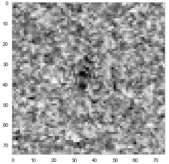
Now that we uderstand the structure and distribution of our data, let's take a look at the images. In the example pics, the contrast between the hh and hv iceberg images is greater than the contrast between the hh and hv ship images. Icebergs seem to "disappear" under hv images, while ships are clearly visible in both hv and hh images. That difference in contrast may have some sort of significance.
band_1_ex = train_df.loc[0, 'band_1']
band_1_ex = np.array(band_1_ex)
band_1_square = band_1_ex.reshape(75, 75)
plt.imshow(band_1_square)
plt.show()

band_2_ex = train_df.loc[0, 'band_2']
band_2_ex = np.array(band_2_ex)
band_2_square = band_2_ex.reshape(75, 75)
plt.imshow(band_2_square)
plt.show()

band_1_ex = train_df.loc[0, 'band_1']
band_2_ex = train_df.loc[0, 'band_2']
band_sub_1 = np.array(band_1_ex)
band_sub_2 = np.array(band_2_ex)
band_sub = band_sub_1 - band_sub_2
band_sub_square = band_sub.reshape(75, 75)
plt.imshow(band_sub_square)
plt.show()

def plot_image_grid(train, band_type, n_row, n_col):
    band = 'band_1'
    if 'HV' in band_type:
        band = 'band_2'
    classification = ''
    # Plot the first 8 eignenvalues
    plt.figure(figsize=(12,12))
    for i in list(range(n_row * n_col)):
    #     for offset in [10, 30,0]:
    #     plt.subplot(n_row, n_col, i + 1)
    #     offset =0
        sat_image = train.loc[i, band]
        sat_image = np.array(sat_image)
        plt.subplot(n_row, n_col, i + 1)
        plt.imshow(sat_image.reshape(75,75))

        if train.loc[i, 'is_iceberg']:
            classification = 'Iceberg'
        else:
            classification = 'Ship'
        title_text = "{0} {1:.0f} {2}".format(classification, train.loc[i, 'inc_angle'], '$^\circ$')
        plt.title(title_text, size=6.5)
        plt.xticks(())
        plt.yticks(())
    plt.suptitle(band_type)
    plt.show()
The individual plots were useful as a first-pass, but to better appreciate the distinguishing features of ship and iceberg images, we're going to need a lot more examples. The grids below show the horizontally and vertically polarized images of ships and icebergs.
plot_image_grid(
    train_df[train_df.is_iceberg==0].reset_index(drop=True),
    'HH Ships',
    7,
    7
)

plot_image_grid(
    train_df[train_df.is_iceberg==0].reset_index(drop=True),
    'HV Ships',
    7,
    7
)

plot_image_grid(
    train_df[train_df.is_iceberg==1].reset_index(drop=True),
    'HH Icebergs',
    7,
    7
)

plot_image_grid(
    train_df[train_df.is_iceberg==1].reset_index(drop=True),
    'HV Icebergs',
    7,
    7
)

Feature Engineering
Need a way to feed the data from the two images into the classifier.
First thought: Subtract the two arrays and use the incidence angle as just another column.
- Turn each band cell into a numpy array
- The whole column can be a higher dimensional array
- Subtract the two arrays
- Turn the inc_angle column into a numpy array
- Concatenate the difference and inc_angle columns
- Feed into algorithm
Second thought: Take average of both images
- Repeat the process above, but average them using vector operations
band_1_arr = train_df.band_1.apply(np.asarray)
band_2_arr = train_df.band_2.apply(np.asarray)
band_diff = band_1_arr - band_2_arr
band_ave = (band_1_arr + band_2_arr)/2.0

band_ave_series = band_ave.apply(pd.Series)
band_diff_series = band_diff.apply(pd.Series)
band_1_df = band_1_arr.apply(pd.Series)
band_2_df = band_2_arr.apply(pd.Series)
band_ave_df = train_df.copy()
band_ave_df.band_1 = band_ave
plot_image_grid(band_ave_df, 'Average Images', 7, 7)

band_diff_df = train_df.copy()
band_diff_df.band_1 = band_diff
plot_image_grid(band_diff_df, 'Difference Images', 7, 7)

Models
In our first pass, we'll compare a random forest classifier to logistic regression and submit the best results. We'll classify 4 different types of images:
- HH
- HV
- Differences
- Averages
After testing our random forest and logistic regression models on the horizontal data, we'll use the better-performing one for the remainder of our exploration.
HH Models
Our HH model had the best log loss, even though its accuracy was lower than the average model. Of course, the difference in accuracy was not significantly different between the models, so further analysis is needed. In the next iteration, I'll implement k-fold cross validation to make up for the higher variance of a train-test-split.
Random Forests
hh_idea = pd.concat((band_1_df, train_df.inc_angle), axis=1)
forest = RandomForestClassifier(random_state=42)

x = hh_idea[hh_idea.inc_angle.isnull()==False].values
y = train_df.loc[train_df.inc_angle.isnull()==False, 'is_iceberg'].values

x_train, x_test, y_train, y_test = train_test_split(x, y, test_size=.3, random_state=42)
forest.fit(x_train, y_train)
pred = forest.predict(x_test)
pred_prob = forest.predict_proba(x_test)
print "Log Loss:", log_loss(y_test, pred_prob, eps=1e-15)
print "Accuracy Score:", accuracy_score(y_test, pred)
print "Classification Report"
print classification_report(y_test, pred)
hh_conf_matrix = confusion_matrix(y_test, pred)
Logistic Regression
hh_idea = pd.concat((band_1_df, train_df.inc_angle), axis=1)
logreg = LogisticRegression(random_state=42)

x = hh_idea[hh_idea.inc_angle.isnull()==False].values
y = train_df.loc[train_df.inc_angle.isnull()==False, 'is_iceberg'].values

x_train, x_test, y_train, y_test = train_test_split(x, y, test_size=.3, random_state=42)
logreg.fit(x_train, y_train)
pred = logreg.predict(x_test)
print "Accuracy Score:", accuracy_score(y_test, pred)
print "Classification Report"
print classification_report(y_test, pred)
hh_conf_matrix = confusion_matrix(y_test, pred)
HV Model
The random forests classifier outperformed logistic regression, so we'll stick with the former going forward. This is just a first pass, so we may return to the logistic model later, but for now, we're only interested in getting a benchmark.
hv_idea = pd.concat((band_2_df, train_df.inc_angle), axis=1)
forest = RandomForestClassifier(random_state=42)

x = hv_idea[hv_idea.inc_angle.isnull()==False].values
y = train_df.loc[train_df.inc_angle.isnull()==False, 'is_iceberg'].values

x_train, x_test, y_train, y_test = train_test_split(x, y, test_size=.3, random_state=42)
forest.fit(x_train, y_train)
pred = forest.predict(x_test)
print "Classification Report"
print classification_report(y_test, pred)
hv_conf_matrix = confusion_matrix(y_test, pred)
Difference Model
This model performed poorly in both accuracy and log loss.
first_idea = pd.concat((band_diff_series, train_df.inc_angle), axis=1)
forest = RandomForestClassifier(random_state=42)

x = first_idea[first_idea.inc_angle.isnull()==False].values
y = train_df.loc[train_df.inc_angle.isnull()==False, 'is_iceberg'].values

x_train, x_test, y_train, y_test = train_test_split(x, y, test_size=.3, random_state=42)
forest.fit(x_train, y_train)
pred = forest.predict(x_test)
print "Classification Report"
print classification_report(y_test, pred)
diff_conf_matrix = confusion_matrix(y_test, pred)
Average Model
Although this model had the best overall validation results, the log loss was worse here than in the HH model. Further investigation is needed before using this model to identify images in our test set.
average_idea = pd.concat((band_ave_series, train_df.inc_angle), axis=1)
forest = RandomForestClassifier(random_state=42)

x = average_idea[average_idea.inc_angle.isnull()==False].values
y = train_df.loc[train_df.inc_angle.isnull()==False, 'is_iceberg'].values

x_train, x_test, y_train, y_test = train_test_split(x, y, test_size=.3, random_state=42)
forest.fit(x_train, y_train)
pred = forest.predict(x_test)
pred_prob = forest.predict_proba(x_test)
print "Log Loss:", log_loss(y_test, pred_prob, eps=1e-15)
print "Accuracy Score:", accuracy_score(y_test, pred)
print "Classification Report"
print classification_report(y_test, pred)
ave_conf_matrix = confusion_matrix(y_test, pred)
def plot_conf_matrix(conf_matrix, title):
    conf_df = pd.DataFrame(conf_matrix)
    conf_df.columns = ['Ship', 'Iceberg']
    conf_df.index = ['Ship', 'Iceberg']

    sns.heatmap(
        conf_df,
        square=True,
        annot=True,
        cmap='viridis',
        fmt='0g'
    )
    plt.ylabel('True Label')
    plt.xlabel('Predicted Label')
    plt.suptitle(title)
    plt.show()
plot_conf_matrix(hh_conf_matrix, 'HH Model')
plot_conf_matrix(hv_conf_matrix, 'HV Model')
plot_conf_matrix(diff_conf_matrix, 'Diff Model')
plot_conf_matrix(ave_conf_matrix, 'Average Model')


Submission 1 (HH Only)
Now that we have our trained classifier, we'll apply it to the test set and prepare our first submission.
Convert band_1 to its own dataframe
band_1_test_arr = test_df.band_1.apply(np.asarray)
band_1_test_df = band_1_test_arr.apply(pd.Series)
Extract inc_angle from test set and concat with band_1
hh_submission = pd.concat((band_1_test_df, test_df.inc_angle), axis=1)
Run predict_proba on array
x = hh_submission.values
pred = forest.predict(x)
pred_prob = forest.predict_proba(x)
Convert pred_prob to dataframe for submission
submission = pd.DataFrame(pred_prob)
submission.columns = ['not_iceberg', 'is_iceberg']
Extract the right column from each predict_proba row
submission = submission.is_iceberg
submission = pd.concat((test_df.id, submission), axis=1)
Check to make sure dataframe is formatted correctly
submission.head()
Convert to csv for submission
submission.to_csv('data/submission_v1.csv', index=False)
Conclusions
This was a fun exploration into image recognition using SAR images. There is still a lot to explore here. We did not tune our hyperparameters and only tested out two models, but we were able to achieve 75% accuracy, which is pretty good for a bunch of fuzzy black and white images. There are still many unexplored feature engineering ideas:
- Combine the two images
- Extract the highest and lowest values from each hh and hv image
- Use PCA for dimensionality reduction
- Use fisher images for dimensionality reduction
- Reduce noise in darker images
- Apply a fourier transform or other transformation technique
I strongly suspect that the difference in polarization scattering is part of key to improving our accuracy, but I'm a little fuzzy on my physics and will need to review some calculus for the fourier transformation. Development on this project will continue over time as we use both domain knowledge and more advanced algorithms (convolutional neural nets) to improve our score. Thank you for taking a look at this analysis.